In this post we will look into how we can train any model using Evolution Strategies (ES) and various advantages of it. We will then build a simple neural network from scratch in Python (by only using numpy) and train it on MNIST Handwritten Digit dataset using ES. This simple implementation will help us understand the concept better and apply it to other settings. Let’s get started!
Table of Content
- Numerical Optimization
- Evolution Strategies
- Vanilla Implementation
- Python Implementation from scratch
- Ending note
Numerical Optimization
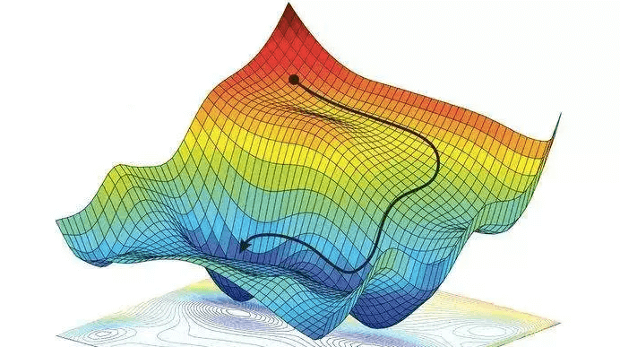
Almost every machine learning algorithm can be posed as an optimization problem. In an ML algorithm, we update the model’s parameters to minimize the loss. For example, every supervised learning algorithm can be written as, $\hat{\theta} = \underset{\theta}{\arg\min} \mathbb {E}_{x,y}[L(y,f(x,\theta))]$, where $x$ and$y$ represent the features and the target respectively, $f$ represents the function we are trying to model,$\theta$ represents model parameters and $L$ represents the Loss function, which measures how good our fit is. Gradient Descent algorithm also known as steepest descent has proven to solve such problems well in most of the cases. It is a first-order iterative algorithm for finding the local minimum of a differentiable function. We take steps proportional to the negative of the gradient of the Loss function at the current point, i.e. $\theta_{new} = \theta_{old} - \alpha*\nabla_{\theta} L(y, f(x, \theta_{old}))$. Newton’s Method is another second-order iterative method which converges in fewer iterations but is computationally expensive as the inverse of second-order derivative of the loss function (Hessian matrix) needs to be calculated, i.e. $\theta_{new} = \theta_{old} - [\nabla_{\theta}^2 L(y, f(x, \theta_{old}))]^{-1}*\nabla_{\theta} L(y, f(x, \theta_{old}))$. We are searching for parameter using the gradients as we believe that it will lead us in the direction where loss will get reduced. But can we search for optimal parameters without calculating any gradients? Actually, there are many ways to solve this problem! There are bunch of different Derivitive-free optimization algorithms (also known as Black-Box optimization).

Evolution Strategies
Gradient descent might not always solve our problems. Why? The answer is local optimum in short. For example in case of sparse reward scenarios in reinforcement learning where agent receives reward at the end of episode, like in chess with end reward as +1 or -1 for winning or losing the game respectively. In case we lose the game, we won’t know whether we played horribly wrong or just made a small mistake. The reward gradient signal is largely uninformative and can get us stuck. Rather than using noisy gradients to update our parameters we can resort to derivative-free techniques such as Evolution Strategies (ES).
In this paper by OpenAI, they show that ES is easier to implement and scale in a distributed computational environment, it does not suffer in case of sparse rewards and has fewer hyperparameters. Moreover, they found out that ES discovered more diverse policies compared to traditional RL algorithm.
ES are nature-inspired optimization methods which use random mutation, recombination, and selection applied to a population of individuals containing candidate solutions in order to evolve iteratively better solutions. It is really useful for non-linear or non-convex continuous optimization problems.
In ES, we don’t care much about the function and its relationship with the inputs or parameters. Some million numbers (parameters of the model) go into the algorithm and it spits out 1 value (eg. loss in supervised setting; reward in case of Reinforcement Learning). We try to find the best set of such numbers which returns good values for our optimization problem. We are optimizing a function $J(\theta)$ with respect to the parameters $\theta$, just by evaluating it without making any assumptions about the structure of $J$, and hence the name ‘black-box optimization’. Let’s dig deep into the implementation details!
Vanilla Implementation
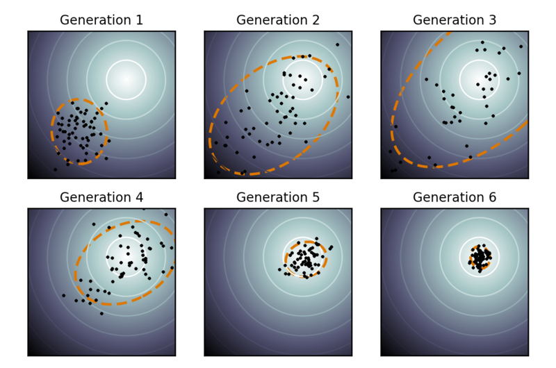
To start with, we randomly generate the parameters and tweak it such that the parameters work better slightly. Mathematically, at each step we take a parameter vector $\theta$ and generate a population of, say, 100 slightly different parameter vectors $\theta_1$ … $\theta_{100}$ by jittering $\theta$ with gaussian noise. We then evaluate each one of the 100 candidates independently by running the model and based on the output value evaluate the loss or the objective function. We then select top N best performing elite parameters, N can be say 10, and take the mean of these parameters and call it our best parameter so far. We then repeat the above process by again generating 100 different parameters by adding gaussian noise to our best parameter obtained so far.
Thinking in terms of natural selection, we are creating a population of parameters (species) randomly and selecting the top parameters that perform well based on our objective function (also known as fitness function). We then take combine the best qualities of these parameters by taking their mean (this is a crude way but it still works!) and call it our best parameter. We then recreate the population by mutating this parameter by adding random noise and repeat the whole process till convergence.

Pseudo Code:
- Randomly initialize the best parameter using a gaussian distribution
- Loop untill convergence:
- Create population of parameters $\theta_1,…\theta_{100}$ by adding gaussian noise to the best parameter
- Evaluate the objective function for all the parameters and select the top N best performing parameters (elite parameters)
- Best parameter = Mean(top N elite parameters)
- Decay the noise at the end of each iteration by some factor (At the start more noise will help us to explore better but as we reach the convergence point we want the noise to be minimum so as to not deviate away)

Python Implementation from scratch
Let’s go through a simple example in Python to get a better understanding. I tried to add details related to numerical stability as well for few of the things. Please read the comments! We will start by loading the required libraries and the MNIST Handwritten digit dataset.
# Importing all the required libraries
import numpy as np
import matplotlib.pyplot as plt
import tqdm
import pickle
import warnings
warnings.filterwarnings('ignore')
from keras.datasets import mnist

# Machine Epsilon (needed to calculate logarithms)
eps = np.finfo(np.float64).eps

# Loading MNIST dataset
(x_train, y_train), (x_test, y_test) = mnist.load_data()

# x contains the images (features to our model)
# y contains the labels 0 to 9

# Normalizing the inputs between 0 and 1
x_train = x_train/255.
x_test = x_test/255.

# Flattening the image as we are using
# dense neural networks
x_train = x_train.reshape( -1, x_train.shape[1]*x_train.shape[2])
x_test = x_test.reshape( -1, x_test.shape[1]*x_test.shape[2])

# Converting to one-hot representation
identity_matrix = np.eye(10)
y_train = identity_matrix[y_train]
y_test = identity_matrix[y_test]

# Plotting the images
fig, ax = plt.subplots(2,5)
for i, ax in enumerate(ax.flatten()):
    im_idx = np.argwhere(y_train == i)[0]
    plottable_image = np.reshape(x_train[im_idx], (28, 28))
    ax.set_axis_off()
    ax.imshow(plottable_image, cmap='gray')

plt.savefig('mnist.jpg')
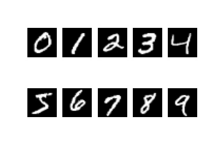
This is how the images look like,

We will start by defining our model, which will be a single layer neural network with only forward pass.
def soft_max(x):

   '''
    Arguments: numpy array

    Returns: numpy array after applying
             softmax function to each
             element
    '''

    # Subtracting max of x from each element of x for numerical
    # stability as this results in the largest argument to
    # exp being 0, ruling out the possibility of overflow
    # Read more about it at :
    # https://www.deeplearningbook.org/contents/numerical.html

    e_x = np.exp(x - np.max(x))

    return e_x /e_x.sum()


class Model():

    '''
    Single layer Neural Network

    '''

    def __init__(self, input_shape, n_classes):

        # Number of output classes
        self.n_classes = n_classes

        # Parameters/Weights of our network which we will be updating
        self.weights = np.random.randn(input_shape, n_classes)

    def forward(self,x):

        '''
        Arguments: numpy array containing the features,
                   expected shape of input  array is
                   (batch size, number of features)


        Returns: numpy array containing the probability,
                 expected shape of output array is
                 (batch size, number of classes)

        '''

        # Multiplying weights with inputs
        x = np.dot(x,self.weights)

        # Applying softmax function on each row
        x = np.apply_along_axis(soft_max, 1, x)

        return x


    def __call__(self,x):

        '''
        This dunder function
        enables your model to be callable


        When the model is called using model(x),
        forward method of the model is called internally

        '''

        return self.forward(x)


    def evaluate(self, x, y, weights = None):

        '''

        Arguments : x - numpy array of shape (batch size,number of features),
                    y - numpy array of shape (batch size,number of classes),
                    weights - numpy array containing the parameters of the model


        Returns : Scalar containing the mean of the categorical cross-entropy loss
                  of the batch


        '''

        if weights is not None:

            self.weights = weights


        # Calculating the negative of cross-entropy loss (since
        # we are maximizing this score)
        # Adding a small value called epsilon
        # to prevent -inf in the output

        log_predicted_y = np.log(self.forward(x) + eps)

        return (log_predicted_y*y).mean()
We will now define our function which will take a model as input and update its parameters.
def optimize(model,x,y,
             top_n = 5, n_pop = 20, n_iter = 10,
             sigma_error = 1, error_weight = 1,  decay_rate = 0.95,
             min_error_weight = 0.01 ):

    '''
    Arguments : model - Model object(single layer neural network here),
               x - numpy array of shape (batch size, number of features),
               y - numpy array of shape (batch size, number of classes),
               top_n - Number of elite parameters to consider for calculating the
                       best parameter by taking mean
               n_pop - Population size of the parameters
               n_iter - Number of iteration
               sigma_error - The standard deviation of errors while creating
                              population from best parameter
               error_weight - Contribution of error for considering new population
               decay_rate - Rate at which the weight of the error will reduce after
                            each iteration, so that we don't deviate away at the
                            point of convergence. It controls the balance between
                            exploration and exploitation


    Returns : Model object with updated parameters/weights

    '''

    # Model weights have been randomly initialized at first
    best_weights = model.weights

    for i in range(n_iter):

        # Generating the population of parameters
        pop_weights = [best_weights + error_weight*sigma_error* \
                       np.random.randn(*model.weights.shape)

                       for i in range(n_pop)]


        # Evaluating the population of parameters
        evaluation_values = [model.evaluate(x,y,weight) for weight in pop_weights]

        # Sorting based on evaluation score
        weight_eval_list = zip(evaluation_values, pop_weights)

        weight_eval_list = sorted(weight_eval_list, key = lambda x: x[0], reverse = True)

        evaluation_values, pop_weights = zip(*weight_eval_list)

        # Taking the mean of the elite parameters
        best_weights = np.stack(pop_weights[:top_n], axis=0).mean(axis=0)

        #Decaying the weight
        error_weight = max(error_weight*decay_rate, min_error_weight)

    model.weights = best_weights

    return model

# Instantiating our model object
model = Model(input_shape= x_train.shape[-1], n_classes= 10)

print("Evaluation on training data", model.evaluate(x_train, y_train))


# Running it for 200 steps
for i in tqdm.tqdm(range(200)):

    model = optimize(model,
                     x_train,
                     y_train,
                     top_n = 10,
                     n_pop = 100,
                     n_iter = 1)

    print("Test data cross-entropy loss: ", -1*model.evaluate(x_test, y_test))
    print("Test Accuracy: ",(np.argmax(model(x_test),axis=1) == y_test).mean())

# Saving the model for later use
with open('model.pickle','wb') as f:
    pickle.dump(model,f)
Results : After training for 200 iterations the test accuracy was ~ 85% and cross-entropy loss was ~ 0.3. This is comparable to a single layer neural network trained with back propagation.
Ending note
ES are very simple to implement and don’t require gradients. Just by injecting noise into our parameters we are able to search the parameter space. Even though we have solved it for a supervised problem for the ease of understanding, it is more suited for Reinforcement learning scenarios where one has to estimate the gradient of the expected reward by sampling. Hope you enjoyed reading this post!
References and further reading: