In this three-part blog series, we will deep dive into the theory and implementation details behind Proximal Policy Optimization (PPO) in PyTorch. In the first part of the series, we will understand what Policy Gradient methods are; in the second part we will look into recent developments in Policy Gradient methods like Trust Regions and Clipped Surrogate Objective to understand how PPO works; in the third part we will go through the detailed implementation of PPO in Pytorch where we will teach an agent to land a rocket in gym’s Lunar Lander environment and also help a Bipedal Walker learn to walk. Let’s get started!

Table of Content

1. Introduction
2. Policy Gradient Methods
3. Baselines
   1. Vanilla Policy Gradient Algorithm
   2. REINFORCE Algorithm
   3. REINFORCE with baseline
   4. Actor - Critic Method
4. Generalized Advantage Estimate (GAE)
5. Ending Note

Introduction

Proximal Policy Optimization(PPO) is a class of policy gradient methods designed by OpenAI that can solve a wide variety of complicated tasks ranging from Atari games, Robotic control to even defeating World Champions at DOTA 2. The main goal for PPO was to address the earlier problems in policy gradient methods by improving upon:

• Ease of implementation
• Sample Efficiency
• Ease of tuning hyperparameters

PPO is a on-policy learning method which doesn’t store past experience and learns on the go. Earlier methods used to perform only one gradient update per data sample making it sample inefficient but PPO enables multiple passes over same data sample making it more sample efficient. PPO also combines the benefits of Trust region policy optimization (TRPO), which is another policy gradient method with reliable performance, but it is much simpler to implement. Similar to TRPO, PPO avoids large policy update and hence provides stable training with lesser number of tweaks. PPO provides the ease of implementation and hyper-parameter tuning along with being sample efficient, while trying to maximize the objective function by updating the policy without deviating much from the earlier one.

To understand PPO, let’s first start with understanding what policy gradient methods are.

Policy Gradient Methods

A lot of the current successes in Deep Reinforcement Learning is because of Policy gradient methods. This is an approach in reinforcement learning where we directly learn the policy to select the best action. We try to find the stochastic policy (probability of taking an action in a given state) that maximizes our expected return (sum of total future rewards with discounting factor). We collect a bunch of trajectories (sequence of states, actions and rewards) with our current policy and try to increase the probability of good trajectories/actions by updating the parameters of our policy.

We can write the parameterized policy as, $\pi (a|s,\theta) = P(A_{t}=a|S_{t} = s, \theta_{t} = \theta)$, i.e., probability that action $a$ is taken at time $t$ given that the environment is in state $s$ at time $t$ with parameter $\theta \in \mathcal{R}^{d} $. We consider a scalar performance measure $J(\theta)$ which is the expected return given current policy i.e. $E[R|\pi_{\theta}]$ where $R$ is the sum of discounted future rewards $r$, $R = \sum_{t=0}^{\infty}\gamma^{t}r_{t}$, $\gamma$ is the discounting factor, generally it is 0.99 (discounting emphasizes recent rewards than future ones, it prevents the sum from blowing up and helps in reducing variance). We try to maximize $J(\theta)$ by updating the parameters using gradient ascent, $\theta_{t+1} = \theta_{t} + \alpha*\widehat{\nabla J(\theta_{t})}$, where $\widehat{\nabla J(\theta_{t})} \in \mathcal{R}^{d}$ is a stochastic estimate (calculated through sampling) whose expectation approximates the gradient of the performance measure with respect to its parameter $\theta$. Let’s understand the math behind it by calculating the gradient of expectation $E_{x\sim p(x|\theta)}[f(x)]$,

\[\nabla_{\theta}E_{x}[f(x)]\\ = \nabla_{\theta}\int p(x|\theta) f(x)dx\\ = \int \nabla_{\theta}p(x|\theta) f(x)dx\\ = \int p(x|\theta)\frac{\nabla_{\theta}p(x|\theta)}{p(x|\theta)} f(x)dx\\ = \int p(x|\theta)\nabla_{\theta}\log p(x|\theta) f(x)dx\\ = E_{x}[ f(x)\nabla_{\theta}\log p(x|\theta)]\]

Here we have used the fact that $\nabla\log f(x) = \frac{\nabla f(x)}{f(x)}$, this converts the integral into expectation, using which we can calculate the integral approximately through sampling. We can sample $N$ such $x_{i}$ from $p(x|\theta)$ and calculate $ f(x_{i}) \nabla_{\theta}\log p(x_{i}|\theta)$ for each $x_{i}$, so the gradient of the expectation will be, \(\nabla_{\theta}E_{x}[f(x)] \approx \sum_{i=0}^{N} (f(x_{i}) \nabla_{\theta}\log p(x_{i}|\theta))/N\) This expression is valid even if the function is discontinuous and unknown, or sample space containing $x$ is a discrete set. This is the beauty of the log derivative trick and now you know why you see log in such objective functions.

Let’s try to understand this gradient expression as it will be the central idea behind policy gradient. The gradient, $\nabla_{\theta}\log p(x_{i},\theta))$ is a vector which gives a direction in the parameter space of $\theta$, and if we move in this direction we will increase the probability of observing $x_{i}$ by changing $p(x_{i}|\theta)$. The final gradient direction is the weighted sum of all the individual gradients (vectors) with $f(x_{i})$ as weights, which means high value of $f(x_{i})$ have more contribution to the final gradient vector. So the probability of observing $x_{i}$ with higher $f(x_{i})$ increases as they have more say in the parameter update. So after updating $\theta$, if we sample from $p(x|\theta)$ it will return $x_{i}$ which have high $f(x_{i})$. This will maximize the expectation $E_{x\sim p(x|\theta)}[f(x)]$, as it roughly translates to the mean of the observed $f(x_{i}) $. Let’s consider a simple example to understand this concept better.

Consider a reward function which takes a real number (e.g. agent’s action) and outputs a reward value for that action. Let’s define an arbitrary reward function $f$, such that $f: \mathcal{R}-> \mathcal{R}$,

$f(x) = 0 $, for $ x <=0$

$f(x) = 2 $, for $ 0< x <=2$

$f(x) = x $, for $ 2< x <=4$

$f(x) = 8 - x $, for $ 4< x <=8$

$f(x) = 0 $, for $ x>8$,

The function looks like this

Reward Function

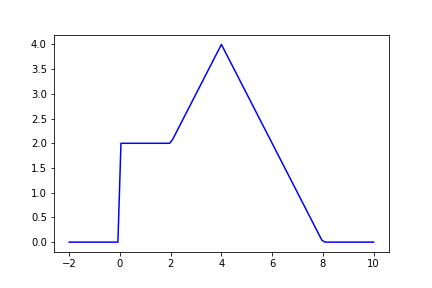
I have chosen an arbitrary function with one peak and some plateau region, to show that we can update the parameters of our probability density function in such a way that we get values closer to the peak (in this case 4) when we sample from this distribution. We can think of the probability density as our policy, we want to have a policy which takes actions that gives higher reward. Let’s do a simulation to understand how the policy evolves to maximize return. We will start with a random Gaussian policy and update it using gradient sampling as mentioned above to get our final policy. Time to look at some code!

#Importing Packages
import numpy as np

# Always set random seeds
# for reproducibility
np.random.seed(0)

import torch
torch.manual_seed(0)
import torch.nn as nn
import torch.optim as optim
from torch.distributions import Normal

import scipy.stats as stats

import matplotlib.pyplot as plt

#Importing celluloid to create animation
from celluloid import Camera
from IPython.display import HTML


class GaussianDistribution(nn.Module):
    
    def __init__(self):
        
        super().__init__()
        
        #Initializing the mean with zeros
        self.mean = nn.Parameter(torch.zeros(1,1))
        
        # Instead of estimating std directly, we 
        # estimate the log of standard deviation, 
        # so that when we take exp of this estimate, 
        # we get the std that way it is always positive
        
        # Initializing the log of std with 1
        self.log_std = nn.Parameter(torch.ones(1,1))
        
    def forward(self):
        
        """
        Returns a Normal distribution
        
        """

        return Normal(self.mean, self.log_std.exp())
    
    
def update_policy(samples=100, 
                  steps = 10, 
                  plot = True,
                  plot_interval = 50):

    
    """
    Arguments: samples - Number of samples to be
                         used for update
                         
               steps - Number updates to the policy
               
               plot - (True/False) Whether to plot or not
               
               plot_interval - Plotting Interval needed 
                               to create animation
                               
    Returns: an animation object
                               
    Description: Updates the 
    
    """
    
    if plot:
        
        fig = plt.figure()

        # Setting up camera to 
        # capture frames for animation
        camera = Camera(fig)

        plt.xlabel('Continuous Action Space')
        plt.title('Policy update to maximize reward')


    # Creating our x-axis
    x = np.linspace(-2, 10, 201)
    
    for i in range(steps):
        
        dist = gaussian_dist()
        
        # Sampling values from our policy
        sampled_values = dist.sample((samples,))
        
        # Getting the log probability for each sample
        log_probs = (dist.log_prob(sampled_values)
                     .flatten())
        
        # Getting the function output for each sample
        func_values = torch.from_numpy(vectorised_my_func(
                                    sampled_values
                                     .flatten()
                                     .numpy()))
        
        # Defining our objective function
        # minus  sign is for maximizing it
        objective_func = -(log_probs*func_values).mean()
        
        # Clearing any past gradient
        # otherwise gradients get accumulated
        optimizer.zero_grad()
        
        # Calculating the gradients of objective
        # function with respect to the parameters
        objective_func.backward()
        
        #Updating the parameters of the policy
        optimizer.step()
        
        # Plotting the policy update
        if plot and i % plot_interval == 0 :
            
            plt.plot(x,stats.norm.pdf(x,
                        gaussian_dist.mean.item(), 
                        gaussian_dist.log_std.exp().item()),
                     color='r')
            
            plt.plot(x, vectorised_my_func(x), color = 'b')
            
            plt.legend(['Policy (Step: %d)'%i,'Reward function'])
            
            camera.snap()
    
    if plot:
        
        plt.close()

        return camera

    return 
        
                                  
# Defining our function
my_func = lambda x: 4-abs(x-4) if 2<=x<=8 else 2 if 0<=x<=2 else 0

# Vectorizing our function so that it can take
# multiple inputs and evaluates them simultaneously

vectorised_my_func = np.vectorize(my_func, otypes = [float])
# CAUTION:
# Don't forget to mention otype (output data type)
# otherwise it infers datatype from the first output value 
# and will convert all the values based on that. For eg. 
# in this case it forces all the output to be integer if we don't
# mention the output type.

# Instantiating our distribution
gaussian_dist = GaussianDistribution()

print('Initial Policy Parameters')
print('Mean:',gaussian_dist.mean.item())
print('Standard Deviation:', gaussian_dist.log_std.exp().item())


# Setting up the Adam optimizer 
optimizer = optim.Adam(gaussian_dist.parameters(), lr= .01 )


# Updating the policy with 100 samples
# for 1000 steps
camera = update_policy(samples= 100, 
                       steps = 1000,
                       plot = True,
                       plot_interval = 50)

print('\nUpdated Policy Parameters')
print('Mean:',gaussian_dist.mean.item())
print('Standard Deviation:', gaussian_dist.log_std.exp().item())

animate = camera.animate()

HTML(animate.to_html5_video())

#Result:
#Initial Policy Parameters
# Mean: 0.0
# Standard Deviation: 2.7182817459106445

# Updated Policy Parameters
# Mean: 4.038374900817871
# Standard Deviation: 0.08744653314352036

In this animation we can see how the policy evolves to maximize the expected value of the function. Since our policy which is a Gaussian distribution has the peak at $x=4$ which coincides with the peak of the function, so when inputs to the function are sampled from this probability distribution and fed to the function, we observe high output values.

In policy gradient method, the random variable $x$ is a whole trajectory $\tau$ which is a sequence of states, actions and rewards, i.e.,

$\tau = (s_{0}, a_{0}, r_{0}, s_{1}, a_{1}, r_{1}, …, …, s_{T -1 }, a_{T-1}, r_{T-1})$,

We will calculate the gradient of expectation (our performance measure) over trajectories ,

$\nabla_{\theta} J(\theta) = \nabla_{\theta}E_{\tau}[R(\tau)] = E_{\tau}[ R(\tau) \nabla_{\theta}\log p(\tau|\theta)]$,

Here $p(\tau|\theta)$ is the probability of trajectory given the parameter $\theta$,

\[p(\tau|\theta) = \mu(s_{0}) \prod_{t=0}^{T-1}[\pi(a_{t}|s_{t},\theta)P(s_{t+1},r_{t}|s_{t},a_{t})]\\ \log p(\tau|\theta) = \log\mu(s_{0})+ \sum_{t=0}^{T-1}[\log\pi(a_{t}|s_{t},\theta)+ \log P(s_{t+1},r_{t}|s_{t},a_{t})]\\ \nabla_{\theta}\log p(\tau|\theta) = \nabla_{\theta}\sum_{t=0}^{T-1}\log\pi(a_{t}|s_{t},\theta)\]

where $\mu(s_{0})$ is the probability of initial state and $P(s_{t+1},r_{t}|s_{t},a_{t})$ is the probability of transitioning from $s_{t}$ to $s_{t+1}$ after taking action $a_{t}$ (this represents the environment dynamics). Both $\nabla_{\theta}\log\mu(s_{0})$ and $\nabla_{\theta}\log P(s_{t+1},r_{t}|s_{t},a_{t})$ are equal to 0 as they don’t depend on $\theta$. Since $\nabla_{\theta}\log P(s_{t+1},r_{t}|s_{t},a_{t})= 0$, that means our algorithm doesn’t care about the system dynamics, even without knowing anything about how the states are transitioning based on our actions, we can still learn. That’s the best part of the algorithm. So now after substituting our gradient becomes,

$\nabla_{\theta} J(\theta) = \nabla_{\theta}E_{\tau}[R(\tau)] = E_{\tau}[R\nabla_{\theta}\sum_{t=0}^{T-1}\log\pi(a_{t}|s_{t},\theta))] $

Let’s understand the intuition behind this gradient. We are trying to maximize our performance measure $J(\theta)$ by increasing probability of good trajectories and decreasing probability of bad trajectories. $\nabla_{\theta}\log\pi(a_{t}|s_{t},\theta))$ gives the direction in which we should move in the parameter space to increase the probability of action at time $t$. Since the final direction is the weighted sum of all vector directions with the Return of the trajectory as weight,.i.e, $\sum_{i = 1}^{N}R(\tau_{i})\nabla_{\theta}\log p(\tau_{i}|\theta)/N$,so if $R$ is higher for a trajectory the final gradient direction will tend to be in direction that maximizes the probability of actions taken in that trajectory and when $R$ is lower it will give lesser weightage to it.

We can improve this gradient further. We know that rewards collected before time $t$ shouldn’t affect the probability of actions taken starting from $t$. Only the current state’s information is required for the agent to take an action and the reward follows from that. So only the future discounted rewards should impact the probability of agent’s actions. Using this fact, we can rewrite the equations as,

$\nabla_{\theta} J(\theta) = \nabla_{\theta}E_{\tau}[R(\tau)] = E_{\tau}[\nabla_{\theta}\sum_{t=0}^{T-1}\log\pi(a_{t}|s_{t},\theta))\sum_{t^\prime=t}^{T-1}\gamma^{t^{\prime}-t}r_{t}]$

There are still couple of problems with this gradient estimation. Do you see it? Suppose $R>=0$, then even if $R$ is small for a trajectory there is a still small positive component that is trying to increase the probability of actions taken during that trajectory. This doesn’t make sense as we should reduce the probability of actions which contribute to small returns. We will encounter same problem with all $R$ being negative. Moreovoer, the gradient estimation has high variance and is noisy which slows down the learning. This is mainly because with small changes in action we may end up in complete different trajectories with different returns. Also, we are only sampling few trajectories out of the possible millions. In the next section we will look at how we can tackle this.

Baselines

To alleviate the problem described in the last part of previous section, we will introduce the concept of baselines. Now the gradient of the performance measure changes to,

$\nabla_{\theta} J(\theta) = \nabla_{\theta}E_{\tau}[R(\tau)] = E_{\tau}[\nabla_{\theta}\sum_{t=0}^{T-1}\log\pi(a_{t}|s_{t},\theta))(\sum_{t^\prime=t}^{T-1}\gamma^{t^{\prime}-t}r_{t}-b)]$, where b is the baseline. Intuitively, we want the baseline to be the average return when we are present in the state and we want to only increase (or decrease) the probability of the action if the observed return is more (or less) than the average. $\hat{A_{t}} = \sum_{t=t^{\prime}}^{T-1}\gamma^{t-t^{\prime}}r_{t} - b$, is called the advantage estimate. Interestingly, this doesn’t change our gradients. We can see why by looking at the part of expected value of the gradient where b is present,

\(E_{\tau}[\nabla_{\theta}\sum_{t=0}^{T-1}\log\pi(a_{t}|s_{t}) b]\\ = E_{\tau}[\nabla_{\theta}\log p(\tau|\theta) b]\\ = \sum_{\tau}[p(\tau|\theta)\frac{\nabla_{\theta}p(\tau|\theta)}{p(\tau|\theta)} b]\\ = b\nabla_{\theta}\sum_{\tau}p(\tau|\theta)\\ =b\nabla_{\theta}1\\ = 0\) So the gradient estimate doesn’t get biased because of the baseline.

You might be wondering, what are the good choices for b?

• It can be a simple constant baseline: $b \approx \frac{1}{N}\sum_{i=1}^{N}R(\tau^{(i)})$, this is just the average return of all the trajectories
• Or, it can be state-dependent expected return: $b(s_{t}) = E[r_{t} + \gamma r_{t+1}…. + \gamma^{T-1-t}r_{T-1}| s_{t}] = V^{\pi}(s_{t})$.

To evaluate $V^{\pi}(s_{t})$, we can have a neural network which takes the state as input and regress it over the target $\sum_{i=t}^{T-1}\gamma^{i-t}r_{t}$ after collecting multiple trajectories. This is the Monte-Carlo estimate of $V^{\pi}(s_{t})$. Steps for Monte-Carlo estimate:

• Initialize $V_{\phi_{0}}^{\pi}$
• Collect Trajectories $\tau_1, \tau_2,…., \tau_m$
• Regress against observed returns \(\phi_{i+1} = \underset{\phi}{\arg\min} \frac{1}{m} \sum_{i=0}^{m}\sum_{t=0}^{H-1}(V_{\phi_{i}}^{\pi}(s_{t}^{(i)}) - \sum_{k=t}^{H-1} R(s_{k}^{(i)}, u_{k}^{(i)}))^2\)

We can also do a Temporal-Difference TD(0) update, by regressing $V^{\pi}(s_{t})$ over $r_{t} + \gamma V^{\pi}(s_{t+1})$ after collecting several samples of $(s_{t}, a_{t}, s_{t+1}, r_{t})$. Motivation for this comes from the Bellman Equation, \(V^{\pi}(s) = \underset{a}\sum \pi(a|s)\underset{s^{\prime}}\sum P(s^{\prime}|s,a)[r(s,a,s^{\prime}) + \gamma V^{\pi}(s^{\prime})]\)

Since we don’t know the transition dynamics ($P(s^{\prime}|s,a)$), so we collect experiences $(s,a,s^{\prime},r)$ using our current policy and average over them to roughly get the expected value. Steps for TD estimate:

• Initialize $V_{\phi_{0}}^{\pi}$
• Collect data $(s,a,s^{\prime},r)$
• Regress against TD target \(\phi_{i+1} = \underset{\phi}{\min} \underset{s,a,s^{\prime},r}\sum || r + \gamma V_{\phi_{i}}^{\pi}(s^{\prime}) -V_{\phi_{i}}^{\pi}(s)||_{2}^{2} + \lambda ||\phi - \phi_{i}||_{2}^{2}\)

The second term in the above loss function ensures our parameter $\phi$ does’t move far from previous estimate $\phi_{i}$.

Let’s look at some of the algorithms.

Vanilla Policy Gradient Algorithm

• Initialize policy parameter $\theta$ and baseline $b$
• For i = 1,2,3… do
  • Collect trajectories by following current policy
  • At each time step in each trajectory, calculate the Return($ R_{t} = \sum_{i=t}^{T-1}\gamma^{i-t}r_{t}$) and advantage estimate ( $\hat{A_{t}} = R_{t} - b(s_{t})$)
  • Update the baseline by minimizing $(b(s_{t})-R_{t})^2$ over all trajectories and timesteps
  • Update the policy using the gradient estimate, $\nabla_{\theta}\sum_{t=0}^{T-1}\log\pi(a_{t}|s_{t},\theta))\hat{A_{t}}$

REINFORCE Algorithm

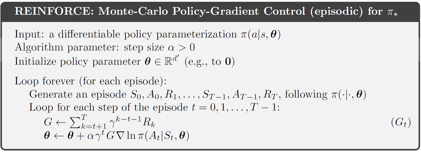
In REINFORCE, we update our policy after a single episode and don’t use baseline. Note: Here $G$ and $R$ are used to denote return and reward respectively.

Source: "Reinforcement Learning" by Richard S. Sutton and Andrew G. Barto

REINFORCE with baseline

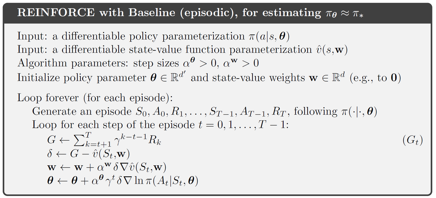
In REINFORCE with baseline, we update our policy after a single episode and use value (expected return for a state) function as our baseline. We update the baseline after each epoch by calculating the gradient of the mean squared error (MSE). Note: Here $G$ and $R$ are used to denote return and rewards respectively.

Source: "Reinforcement Learning" by Richard S. Sutton and Andrew G. Barto

Actor - Critic Method

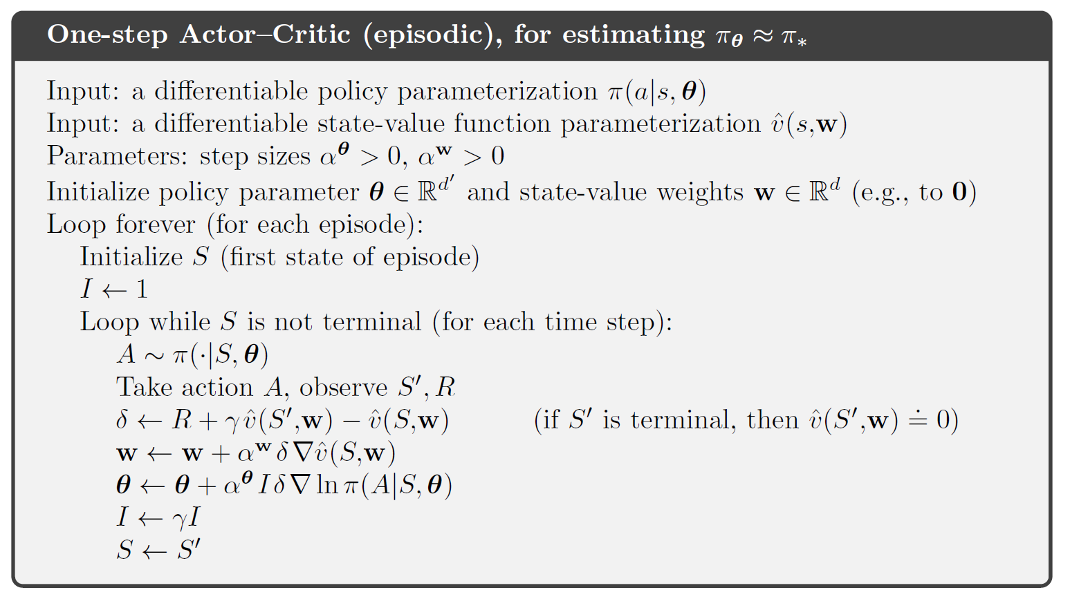
In Actor-Critic Method, the value estimate is updated using the estimate of the subsequent states. This introduces bias and also reduces variance. We will look into it in the next section. Note: Here $G$ and $R$ are used to denote return and rewards respectively.

Source: "Reinforcement Learning" by Richard S. Sutton and Andrew G. Barto

Generalized Advantage Estimate (GAE)

In policy gradient, we want to increase the probability of action which gives us high return for that state. $Q^{\pi}(s_{t},a_{t}) = E[r_{0} + \gamma r_{1} + \gamma^2 r_{2} …|s_{t},a_{t}]$ is the expected return for our current state and action. From a single rollout $R(s_{t}, a_{t}) = \sum_{i=t}^{T-1}\gamma^{i-t}r_{t}$, we obtain the estimation of $Q^{\pi}(s,a) = E[r_{0} + \gamma r_{1} + \gamma^2 r_{2} …| s_{0}=s,a_{0}=a]$, but this will vary across trajectories and will have high variance, hence convergence may be slow. To reduce variance we can introduce function approximation,

\[Q^{\pi}(s,a) = E[r_{0} + \gamma r_{1} + \gamma^2 r_{2} ...| s_{0}=s,a_{0}=a]\\ = E[r_{0} + \gamma V^{\pi}(s_{1})| s_{0}=s,a_{0}=a]\]

or we can take more steps,

\[= E[r_{0} +\gamma r_{1} + \gamma^2 V^{\pi}(s_{2})| s_{0}=s,a_{0}=a]\\ = E[r_{0} +\gamma r_{1} + \gamma^2 r_{2} + \gamma^3 V^{\pi}(s_{3})| s_{0}=s,a_{0}=a]\\ = ....\]

When we take 1 step, i.e. Temporal-Difference TD(0), we are reducing the variance as $V^{\pi}(s)$ (estimated return at state $s$) won’t change across trajectories unless we update it, but it increases our bias as we are estimating the expected return for current state and action using another estimate and not from the observed value. Initially we start our $V^{\pi}(s)$ with random guess and it updates slowly from experience which may not give us the true picture, hence it is biased. When we take all the steps till T-1, we are essentially using Monte-Carlo which is unbiased but high variance as the whole trajectory may be completely different with different returns because of small changes in action selection or state transitioning. The more sampled reward terms we consider more will be our variance because of the noise in them. The good thing about Monte-Carlo is that we have guaranteed convergence and also it is unbiased as we are estimating it from the observed rewards.

Source: David Silver's Lecture Slides (link in references)

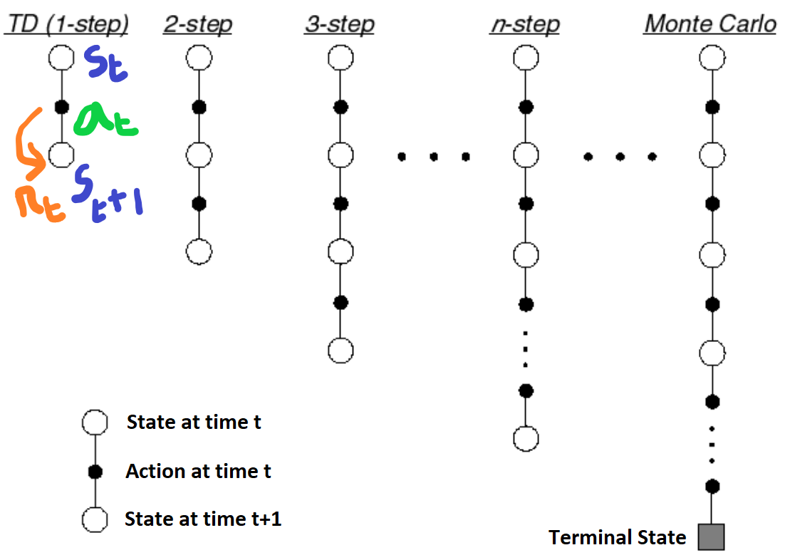
What if there was a way to strike a balance between the two? The answer to that is Generalized Advantage Estimate (GAE). In GAE, we take the weighted sum of all the different step estimates to create the final estimate. Let the $k$-step Advantage estimate be $ \hat{A}_{t}^{(k)} = r_{t} +\gamma r_{t+1} + \gamma^2 r_{t+2}+… +\gamma^{k-1} r_{t+k-1}+ \gamma^{k} V(s_{t+k}) - V(s_{t}) $ and the TD residual be $\delta_{t}^{V} = \hat{A}_{t}^{(1)} = r_{t} +\gamma V^{\pi}(s_{t+1}) - V(s_{t}) $, then the generalized advantage estimate $GAE(\gamma,\lambda)$ is defined as ,

\[\hat{A}_{t}^{GAE(\gamma,\lambda)} = (1-\lambda)(\hat{A}_{t}^{(1)} + \lambda \hat{A}_{t}^{(2)} + \lambda^2 \hat{A}_{t}^{(3)} + ...)\\ = (1-\lambda)( \delta_{t}^{V} + \lambda (\delta_{t}^{V} + \gamma \delta_{t+1}^{V}) +\lambda^2(\delta_{t}^{V} + \gamma \delta_{t+1}^{V} + \gamma^2 \delta_{t+2}^{V}) + ....)\\ = (1-\lambda)( \delta_{t}^{V} (1 + \lambda +\lambda^2 +\lambda^3 +...) + \gamma \delta_{t+1}^{V} (\lambda +\lambda^2 +\lambda^3 +...) + \gamma^2 \delta_{t+2}^{V} (\lambda^2 +\lambda^3 + \lambda^4 ...) + ...)\\ = (1-\lambda)(\delta_{t}^{V}(\frac{1}{(1-\lambda)} + \gamma \delta_{t+1}^{V}(\frac{\lambda}{(1-\lambda)}) + \gamma^2 \delta_{t+2}^{V}(\frac{\lambda^2}{(1-\lambda)} + ...)\\ = \sum_{l=0}^{\infty} (\gamma \lambda)^l \delta_{t+l}^{V}\]

The equation uses the fact that \(\hat{A}_{t}^{(2)} = r_{t} +\gamma r_{t+1} + \gamma^2 V(s_{t+2}) - V(s_{t}) \\ = r_{t} + \gamma V(s_{t+1}) - V(s_{t}) +\gamma (r_{t+1} + \gamma V(s_{t+2}) - V(s_{t+1})) \\ = \delta_{t}^{V} + \gamma \delta_{t+1}^{V}\)

and similarly for other terms. The generalized advantage estimator introduces trade-off between bias and variance, controlled by parameter $\lambda$ when $0<\lambda<1$. There are two extreme cases when $\lambda=0$ and $\lambda=1$. When $\lambda=0$, $GAE(\gamma,0) = r_{t} + \gamma V(s_{t+1}) - V(s_{t})$, it is same as Temporal Difference TD(0) method and when $\lambda=1$ $GAE(\gamma,1) = \sum_{l=0}^{\infty}\gamma^l r_{t+l} - V(s_{t})$, it becomes Monte Carlo method. So by selecting a suitable value of $\lambda$ we can reduce the variance (0.99 works well in practice).

Ending Note

In this post we learnt the mathematics behind Policy Gradient methods and various modifications to reduce variance of the gradients and speed-up learning. In part 2, we will learn how we can improve sample efficiency and make the learning algorithm more reliable through Importance Sampling, Trust Regions and Clipped Surrogate methods. These are some of the core ideas in PPO. In part 3, we will learn to build our own agent from scratch and train it using PPO in Pytorch.

Hope you enjoyed reading the post!

References and Further Reading:

• Deep RL Bootcamp Lecture 4A: Policy Gradients
• David Silver’s Lecture Slides
• Andrej Karpathy’s Blog
• “Reinforcement Learning” by Richard S. Sutton and Andrew G. Barto
• High-Dimensional Continuous Control Using Generalized Advantage Estimation

---

• ← Previous Post
• Next Post →