DRAFT:
Welcome to the second part of this three-part blog series where we deep dive into the theory and implementation details behind Proximal Policy Optimization (PPO) in PyTorch. In the first part of the series, we understood what Policy Gradient methods are; in the second part we will look into recent developments in Policy Gradient methods like Trust Regions and Clipped Surrogate Objective to understand how PPO works; in the third part we will go through the detailed implementation of PPO in Pytorch where we will teach an agent to land a rocket in gym’s Lunar Lander environment and also help a Bipedal Walker learn to walk. Let’s get started!
Table of Content
- Limitations of Vanilla Policy Gradient Methods
- Importance Sampling
- Importance Sampling Interpretation of Policy Gradient Methods
- Trust Region
- Trust Region Policy Optimization (TRPO)
- Clipped Surrogate Objective
In case you have missed the first part, click here. So far we have looked into what policy gradient methods are and how we can use various baselines to reduce variance which gives rise to different methods. In this part, we will look into what makes PPO sample efficient and helps it to deliver reliable performance without much hyperparameter tuning. We will start with understanding the limitations of vanilla policy gradient methods and then go through the various improvements that led the development of PPO.
Limitations of Vanilla Policy Gradient Methods
Step size
In policy gradient methods, the input data is non-stationary due the changing policy which in turn changes observation and reward distribution. This makes it hard to take different step sizes for getting good policy while optimizing the parameters. Initially, if we have a bad policy then we might have to take big step sizes but later on we need to reduce our step size as we don’t want to deviate from the good policy. There is no consistent good step size that works throughout the learning process which makes it hard.
Step too far → Bad Policy → Bad Input Data → Difficult or no recovery
Sample Efficiency
We use data sample only once to calculate a single gradient step for model parameter update. We don’t use all the available information out of it. For example, we may have some small gradients in our parameter update because of poor scaling of features, then we would make very little progress on the parameters with tiny gradients and hence slow learning
Machine learning is all about reducing learning to numerical optimization. If we can change the loss function that we are optimizing we might be able to find solutions to these problems. Let’s start with rewriting the objective function using importance sampling to tackle these issues. But what is Importance Sampling?
Importance Sampling
The name is misleading as it is an approximation technique and not a sampling method. Definition from Wikipedia: It is used to estimate properties of a particular distribution while only having samples generated from a different distribution than the distribution of interest. Let’s look at it in more details, suppose we have want to estimate the expectation of function $f$ when its input $X_{i}$ are drawn from a distribution with probability density $p$. To do that we can generate the sample and take the average of those, i.e. $E[f(x)] \approx 1/N *\sum_{i=1}^{N} f(X_{i})$, where $ X_{i} \sim p$
But what if it is difficult to generate samples from p. There is a clever workaround for this. So instead of drawing samples from $p$ we draw samples from a known density $q$ and using the following trick we can easily calculate the expectation with respect to $p$.
\(E_{x\sim p}[f(x)] = \int f(x)p(x)dx = \int f(x)\frac{p(x)}{q(x)}q(x)dx\) \(\approx 1/N *\sum_{i=1}^{N} f(X_{i})\frac{p(X_{i})}{q(X_{i})}, \text{where } X_{i} \sim q\)
,we can only do this if $q(x) = 0 \implies p(x) = 0$
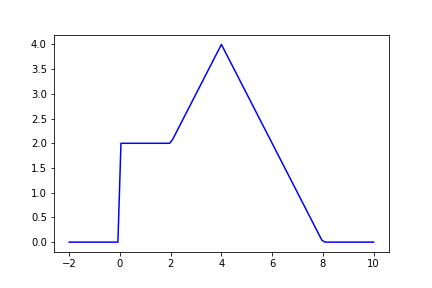
Let’s look at an example, suppose we want to estimate the expectation of an arbitary function $f$ (same function from part 1), such that $f: \mathcal{R}-> \mathcal{R}$,
$f(x) = 0 $, for $ x <=0$
$f(x) = 2 $, for $ 0< x <=2$
$f(x) = x $, for $ 2< x <=4$
$f(x) = 8 - x $, for $ 4< x <=8$
$f(x) = 0 $, for $ x>8$,
Now, we want to estimate its expectation using a gaussian distribution with mean of 4 and standard deviation of 2, $p\sim \mathcal{N}(4, 4)$. For simplicity, assume we don’t have access to this distribution but a different gaussian distribution with mean of 6 and standard deviation of 2, $q\sim \mathcal{N}(6, 4)$. Since we can’t use $p$ so we will use $q$ to get the samples and make the required corrections to our estimate calculation as shown in the equations above. Let’s look at the implementation and results.
import matplotlib.pyplot as plt
import numpy as np
import pandas as pd
import seaborn as sns
np.random.seed(0)

# Our function
def my_func(x):

    if 0 <= x <= 2 :
        return 2

    elif 2 <= x <= 8:
        return 4 - abs(x - 4)

    return 0

# Vectorizing our function to accept
# multiple inputs
my_func = np.vectorize(my_func, otypes=[float])

x = np.linspace(-2, 10, 201)

plt.plot(x, my_func(x))
# Gaussian Distribution
def gaussian(mean, std):

    def _gaussian(x):

        return np.exp(-1 / 2 * ((x - mean) / std)**2)/\
               (std * np.sqrt(2 * np.pi))

    return np.vectorize(_gaussian, otypes=[float])

# Run multiple times to analyze the result
def run():

    # Defining the parameters for the
    # gaussian distributions
    mean_p, std_p = 4, 2
    mean_q, std_q = 6, 2
    N = 1000  # Number of samples

    gaussian_p = gaussian(mean_p, std_p)
    gaussian_q = gaussian(mean_q, std_q)

    # Generating samples
    samples_q = np.random.normal(loc=mean_q,
                                 scale=std_q,
                                 size=N)

    # Calculating expectation using importance sampling
    exp_p_imp_sampling = (my_func(samples_q) * gaussian_p(samples_q)\
                          /(gaussian_q(samples_q) + 1e-7)).mean()

    # Generating samples from p to compare the results against
    # importance samples. NOTE: This has been calculated only
    # for comparison
    samples_p = np.random.normal(loc = mean_p,
                                 scale = std_p,
                                 size = N)

    exp_p = my_func(samples_p).mean()

    return exp_p_imp_sampling, exp_p

# Repeating the experiments to analyze results
repeated_experiment = [run() for i in range(1000)]

imp_sampling_estimate, actual_samples_estimate = \
zip(*repeated_experiment)

# Calculating the difference for each run
differences = [imp_sampling_estimate[i]-actual_samples_estimate[i]
                for i in range(len(repeated_experiment))]

fig, axes = plt.subplots(1,2, figsize = (12,3))

sns.distplot(imp_sampling_estimate,
             label= 'Importance Sampling',
             ax=axes[0])

sns.distplot(actual_samples_estimate,
             label = 'Actual Sampling',
             ax=axes[0])

axes[0].set_title('Distribution of Estimates')
axes[0].legend()

sns.distplot(differences,
            ax = axes[1])

axes[1].set_title('Distribution of difference')
plt.savefig("./importance_sampling.png")
plt.show()
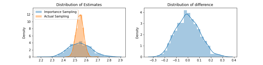
The results look good, the estimates are really close. In this case, the importance sampling estimates have higher variance but if we are free to choose $q$, an optimized choice of $q$ can give us better estimates.
Now, we know what importance sampling is. The only thing remaining is to find out how we can use this to rewrite policy gradient optimization problem to solve the previously mentioned issues.
Importance Sampling Interpretation of Policy Gradient Methods
In policy gradient method, we try to directly maximize the expected advantage estimate, i.e. $E_t[\hat{A}_t]$ (please check part 1 for details). Another way to look at the objective function is that, we collect data using some policy $\pi_{\theta_{old}}$ and we want our updated new policy $\pi_\theta$ to have high advantage estimate, i.e,
\[E_{s_t\sim \pi_{\theta_{old}}, a_t\sim \pi_{\theta}}[A^\pi(s_t, a_t)]\] \[= E_{s_t\sim \pi_{\theta_{old}}, a_t\sim \pi_{\theta_{old}}}[\frac{\pi_\theta(a_t|s_t)}{\pi_{\theta_{old}}(a_t|s_t)}A^{\pi_{\theta_{old}}}(s_t, a_t)]\] \[= E_{s_t\sim \pi_{\theta_{old}}, a_t\sim \pi_{\theta_{old}}}[\frac{\pi_\theta(a_t|s_t)}{\pi_{\theta_{old}}(a_t|s_t)}\hat{A}_{t})]\]To draw analogy with our earlier example of importance sampling, $\pi_{\theta_{old}}$ is our $q$ and $\pi_\theta$ is our $p$, and advantage estimate $\hat{A}_t$ is our function $f$. NEED TO CHECK: This formulation helps us to optimize the parameters and obtain a better new policy using data collected from old policy. We can go over the collected data samples multiple times during gradient update and use all the information, instead of just using it once. There is still one problem remaining. Do you see it? We can’t just take the old policy and keep updating the parameters based on that. We need to be cautious of the step sizes that we take because the training might become unstable as mentioned earlier. One way to solve it is using trust regions.
Trust Region
This is a method in optimization where we use a model or a local approximation of the function we are trying to optimize. We only optimize using this approximation inside a region where it is close to the original function, this region is called the trust region. The local approximation of function is accurate near the starting point but gets inaccurate if we get too far from starting the point, so we have trust regions where we trust our approximation. Let’s look at it in more details, suppose we want to optimize the function $f$ at $x_k$ such that $f(x_{k+1}) < f(x_k)$. To solve this we can create a model $m_k$ using Taylor-series expansion of $f$ around $x_k$, which is, \(f(x_k+p) = f(x_k) + \nabla f(x_k)^Tp+ \frac{1}{2}p^T\nabla^2f(x_k + tp)p, \text{where t} \in (0,1)\)
\[m_k(p) = f(x_k) + \nabla f(x_k)^Tp+ \frac{1}{2}p^T\nabla^2f(x_k)p\]To obtain the next step $x_{k+1}$ we solve the following subproblem, \(\underset{p\in\mathbb{R}^n} \min m_k(p) = f(x_k) + \nabla f(x_k)^Tp+ \frac{1}{2}p^T\nabla^2f(x_k)p\) such that $\lvert \lvert p \rvert\rvert<= \Delta_{k}$, where $\Delta_{k}>0$ is the trust-region radius. One of the most important element here is choosing the trust region, if we don’t get significant reduction in the function value, we reduce the trust region and solve the subproblem again. Next we will see how using the trust region approach we can limit having large updates to our policy.
Trust Region Policy Optimization (TRPO)
To define the trust region, we use KL divergence to measure how far we are from the starting point which is the old policy and our new point which is the new policy. Basically we are trying to limit the change in probabilities using the trust region. So after incorporating this knowledge to our importance sampling interpretation, the constrained objective function looks like this:
\[\underset{\theta}\max \hat{E_t}[\frac{\pi_{\theta}(a_t|s_t)}{\pi_{\theta_{old}}}(a_t|s_t)\hat{A}_t]\]subject to $\hat{E_t}[KL[\pi_{\theta_{old}}(\cdot|s_t), \pi_\theta(\cdot|s_t)]]<= \delta$
and the penalized or unconstrained version looks like this:
\(\underset{\theta}\max \hat{E_t}[\frac{\pi_{\theta}(a_t\|s_t)}{\pi_{\theta_{old}}}(a_t\|s_t)\hat{A}\_t]-\beta\hat{E_t}[KL[\pi_{\theta_{old}}(\cdot\|s_t), \pi_\theta(\cdot\|s_t)]]\), for some coefficient $\beta$
Quoting lines from the paper Proximal Policy Optimization Algorithms: “TRPO uses a hard constraint rather than a penalty because it is hard to choose a single value of that performs well across different problems—or even within a single problem, where the the characteristics change over the course of learning. Hence, to achieve our goal of a first-order algorithm that emulates the monotonic improvement of TRPO, experiments show that it is not sufficient to simply choose a fixed penalty coefficient and optimize the penalized objective Equation with SGD; additional modifications are required”
TRPO tends to give monotonic improvement, with little tuning of hyperparameters and is effective for optimizing large nonlinear policies such as neural networks. Let’s look at the pseudo code to understand it in more details.
For iteration=1, 2, 3,… do:
Run policy for T timesteps or N trajectories Estimate advantage function at all timesteps
\(\underset{\theta} \max \sum_{n=1}^N\frac{\pi_{\theta}(a_n|s_n)}{\pi_{\theta_{old}}(a_n|s_n)}\hat{A}_n\) \(\text{subject to }KL_{\pi_{\theta_{old}}}(\pi_{\theta}) <= \delta\)
end for
This can be efficiently solved by using conjugate gradient descent
Even though TRPO has robust performance compared to other methods, it also has some limitations (source):
- Hard to use with architectures with multiple outputs, e.g. policy and value function (need to weigh different terms in distance metrics)
- Performs poorly on tasks requiring Deep Convolutional Neural Networks (CNN) and Recurrent Neural Networks (RNN), eg. Atari benchmark
- Conjugate gradient makes the implementation complicated
KL Divergence constraint provides nice behaviour in terms of optimization but it also comes with additional computational overhead. It would be nice if we can find a simpler objective function
Clipped Surrogate Objective
The important contribution in PPO is the use of the following objective function, which has the benefits of TRPO, but with simpler implementation and better sample efficiency.
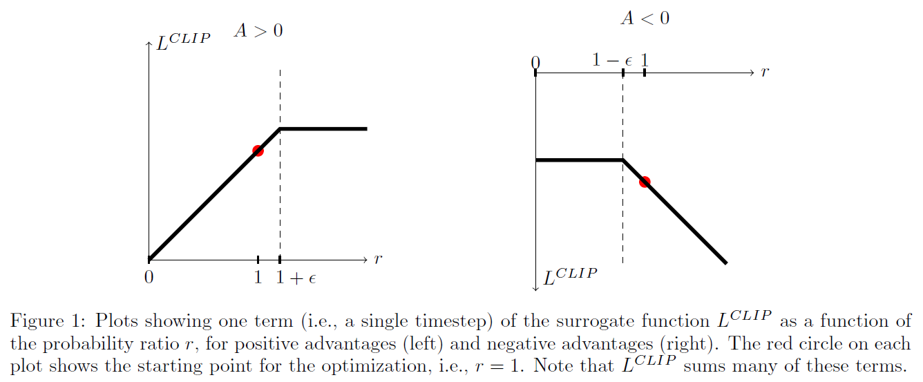
Let $r_t (\theta) = \frac{\pi_{\theta}(a_t|s_t)}{\pi_{\theta_{old}}(a_t|s_t)}$ be the probability ratio
$L^{CLIP} (\theta) = \hat{E_t}[min(r_t(\theta)\hat{A_t}, clip(r_t(\theta), 1-\epsilon, 1+\epsilon)\hat{A_t}]$ , where epsilon is a hyperparameter (e.g. $\epsilon$ = 0.2)
The first term inside $\min$ is our usual objective function and the second the term is the clipped probability ratio whose range is 1-$\epsilon$ to 1+$\epsilon$. We take the minimum of the two so the final clipped objective is a lower bound of the unclipped objective function. In the figure below, we can see that when the Advantage is positive and we need to increase our probability of current actions for better performance, thus increase the probability ratio, but the upper clip prevents the ratio from becoming greater than 1+$\epsilon$, because of the flat objective there will be 0 gradient and hence no update.This way we never move too far from our original policy and can perform multiple gradient updates to obtain better sample efficiency. Similarly, when the advantage is negative and we need to decrease the probability of the current actions, but the lower clip prevents us to move below 1-$\epsilon$. The advantage estimate is gnerally noise so we don’t want to make updates that take our new policy too far from original policy based on single update. When the ratio lies in the slanted region of the clipped objective function, we are basically dealing with the original unclipped objective in this region.
References and Further Reading:
- Deep RL Bootcamp Lecture 4A: Policy Gradients
- Proximal Policy Optimization paper
- Trust Region Policy Optimization paper